مرحبا هبر! من خلال مهنتي الرئيسية ، أنا مهندس تطوير حقول النفط والغاز. أنا فقط أغوص في Data Sciense وهذا هو أول منشور لي أود أن أشارك فيه تجربتي مع التعلم الآلي في صناعة النفط.

يعد توقع إنتاج النفط والغاز بواسطة الآبار من أهم الأمور في صناعة النفط والغاز. بدون توقعات إنتاجية جيدة ، من المستحيل اتخاذ قرارات بشأن ربحية المشاريع ، والاستثمارات الرأسمالية ، وحفر التخطيط الجديد والتشغيلي لتشغيل الآبار القائمة.
في هذه المقالة ، أريد أن أشارك تجربتي في إنشاء نموذج التعلم الآلي لصناعة النفط والغاز. كان الهدف من المبنى النموذجي هو التنبؤ بأحد معايير أداء البئر واختبار قدرة النموذج على التنبؤ بقطع المياه من الآبار الموجودة والآبار المخطط حفرها (مرشحة للحفر).
بيانات الإنتاج هي في الواقع سلسلة زمنية ، مما يشير إلى نموذج أكثر تعقيدًا. من أجل التبسيط والتسريع ، تقرر بناء نموذج لتاريخ محدد.
:
( + ) () () , .
( ). () . , , - - , .
, , . .
3D ().
, ( ). . , . . . . 10 - 15 . , 3- 250 - 1000 . , , " ".
. . . - , . - 3- ( , ) ( ). . , .
. .
:
( , , /- , , ..),
- , , .
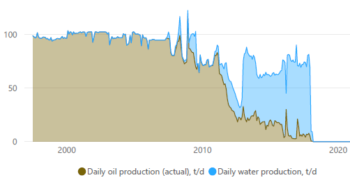
. . , . , . , - . .. Q/(Q + Q)*100%
( ) :
:
Cum oil:
Days: ( ( ) ).
In prod: /
Q oil:
wct:
Top perf: -
Bottom perf:
ST: 0 - , 1 -
x, y:
import numpy as np
import pandas as pd
import matplotlib.pyplot as plt
%matplotlib inline
%config InlineBackend.figure_format = 'svg'
import pylab
from pylab import rcParams
import plotly.express as px
import plotly.graph_objects as go
from sklearn.model_selection import train_test_split
from sklearn.ensemble import RandomForestRegressor
from sklearn.metrics import r2_score as r2, mean_absolute_error as mae, mean_squared_error as mse, accuracy_score
from sklearn.metrics.pairwise import euclidean_distances
.
data_path = 'art_df.xlsx'
df = pd.read_excel(data_path, sheet_name='artificial')
df

- . ( ).
ax = df.plot(kind='scatter', x='x', y='y')
df[['x','y','Well']].apply(lambda row: ax.text(*row),axis=1);
rcParams['figure.figsize'] = [11, 8]
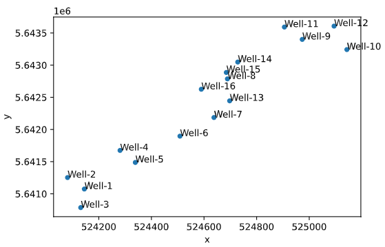
, " " . . , , .
.
distance = pd.DataFrame(euclidean_distances(df[['x', 'y']]))
distance
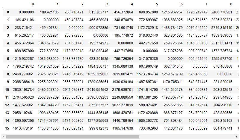
. .
well_names = df['Well']
distance.columns = well_names
. - , .
df_distance = pd.concat([df.drop(['x', 'y'], axis=1), distance], axis=1)
df_distance
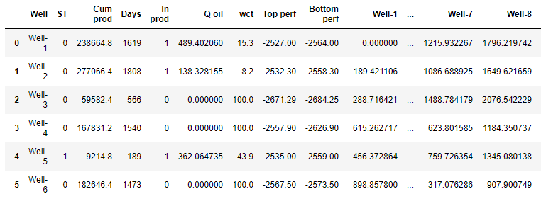
. , ,
df_train_1 = df_distance.drop([12, 13, 14, 15], axis=0)
df_train_1

df_test_1 = df_distance.loc[[12, 13]]
df_test_1

DataFrame X_1. ( ) wct.
x_1 = df_train_1.drop(['Well', 'wct'], axis=1)
x_1

y_1
y_1 = df_train_1['wct']
y_test_1
y_test_1 = df_test_1['wct']
Random Forest Reggressor, , .
x_test_1 = df_test_1.drop(['Well', 'wct'], axis=1)
model = RandomForestRegressor(random_state=42, max_depth=14)
model.fit(x_1, y_1)
y_pred_train_1 = model.predict(x_1)
y_pred_1 = model.predict(x_test_1)
print('Predicted values from train data:')
r2_train = r2(y_1, y_pred_train_1)
mae_train = mae(y_1, y_pred_train_1)
mse_train = mse(y_1, y_pred_train_1)
print(f'R2 train: {r2_train.round(4)}')
print(f'MAE train: {mae_train.round(4)}')
print(f'MSE train: {mse_train.round(4)}')
print('Predicted values from test data:')
r2_test = r2(y_test_1, y_pred_1)
mae_test = mae(y_test_1, y_pred_1)
mse_test = mse(y_test_1, y_pred_1)
print(f'R2 test: {r2_test.round(4)}')
print(f'MAE test: {mae_test.round(4)}')
print(f'MSE test: {mse_test.round(4)}')
model
Predicted values from train data:
R2 train: 0.8832
MAE train: 8.2855
MSE train: 131.1208
Predicted values from test data:
R2 test: 0.8758
MAE test: 3.164
MSE test: 11.4485
RandomForestRegressor(max_depth=14, random_state=42)
R2 R2 1%. , .
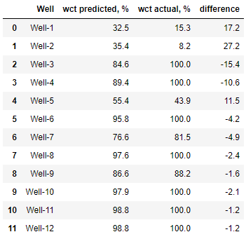
, (blind test)
df_y_test = pd.DataFrame({'Well': df_test_1['Well'],
'wct predicted, %': y_pred_1.round(1),
'wct actual, %': y_test_1.round(1),
'difference': (y_pred_1 - y_test_1).round(1)})
df_y_test

df_y_train = pd.DataFrame({'Well': df_train_1['Well'],
'wct predicted, %': y_pred_train_1.round(1),
'wct actual, %': y_1.round(1),
'difference': (y_pred_train_1 - y_1).round(1)})
df_y_train
:
round(sum(abs(y_pred_train_1 - y_1)) / len(y_1), 1)
8.3
, 8%, .
, ,
df_train_2 = df_distance.drop([14, 15], axis=0)
, .
WCT () = NaN.
df_fc = df_distance.loc[[14, 15]]
DataFrame x_2. ( ) wct.
x_2 = df_train_2.drop(['Well', 'wct'], axis=1)
y_2 .
y_2 = df_train_2['wct']
x_fc = df_fc.drop(['Well', 'wct'], axis=1)
model = RandomForestRegressor(random_state=42, max_depth=14)
model.fit(x_2, y_2)
y_pred_train_2 = model.predict(x_2)
y_fc = model.predict(x_fc)
print('Predicted values from train data:')
r2_train = r2(y_2, y_pred_train_2)
mae_train = mae(y_2, y_pred_train_2)
mse_train = mse(y_2, y_pred_train_2)
print(f'R2 train: {r2_train.round(4)}')
print(f'MAE train: {mae_train.round(4)}')
print(f'MSE train: {mse_train.round(4)}')
print('Forecasted values could be compared with real data!')
model
Predicted values from train data:
R2 train: 0.9095
MAE train: 6.5196
MSE train: 89.9625
RandomForestRegressor(max_depth=14, random_state=42)
R2 .
.
df_y_train = pd.DataFrame({'Well': df_train_2['Well'],
'wct predicted, %': y_pred_train_2.round(1),
'wct actual, %': y_2.round(1),
'difference': (y_pred_train_2 - y_2).round(1)})
df_y_train
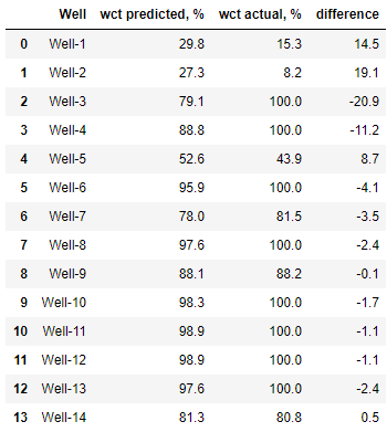
round(sum(abs(y_pred_train_2 - y_2)) / len(y_2), 1)
6,5
6,5. !
:
df_y_test = pd.DataFrame({'Well': df_test_1['Well'],
'wct predicted, %': y_pred_1.round(1),
'wct actual, %': y_test_1.round(1),
'difference': (y_pred_1 - y_test_1).round(1)})
df_y_test

.
model.feature_importances_
feature_importances = pd.DataFrame()
feature_importances['feature_name'] = x_2.columns.tolist()
feature_importances['importance'] = model.feature_importances_
feature_importances = feature_importances.sort_values(by='importance', ascending=False)
feature_importances
fig = px.bar(feature_importances,
x=feature_importances['importance'],
y=feature_importances['feature_name'],
title="Feature importances")
fig.update_layout(yaxis={'categoryorder':'total ascending'})
fig.show()
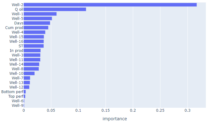
, - 2- . .
. - .
fig = px.scatter(x=y_pred_train_2, y=y_2, title="True vs Predicted values",
text=df_train_2['Well'], width=850, height=800)
fig.add_trace(go.Scatter(x=[0,100], y=[0,100], mode='lines', name='True=Predicted',
line = dict(color='red', width=1, dash='dash')))
fig.update_xaxes(title_text='Predicted')
fig.update_yaxes(title_text='True')
fig.show()

. (- ), (, ).
, " " . , , .
. - "" - .

. " ", . "" . . , .
, . , .
بيانات الآبار ليست بيانات مفتوحة ، بل هي ملك للشركة الحائزة على ترخيص تطوير الحقل. لذلك ، لتوضيح العمل المنجز ، تم إنشاء بيانات بئر اصطناعية متوفرة لهذا العمل.
يتوفر كود المصدر مع نص المقالة هنا: https://github.com/alex-kalinichenko/re/tree/master/wct_fc